2.3 Rates of Change and Behavior of Graphs

Terri Manthey

2.3 Rates of Change and Behavior of Graphs

Since functions represent how an output quantity varies with an input quantity, it is natural to ask about the rate at which the values of the function are changing.

For example, the function $C(t)$ below gives the average cost, in dollars, of a gallon of gasoline $t$ years after 2000.

t	2	3	4	5	6	7	8	9
C(t)	1.47	1.69	1.94	2.30	2.51	2.64	3.01	2.14

If we were interested in how the gas prices had changed between 2002 and 2009, we could computer that the cost per gallon had increased from $1.47 to $2.14, an increase of 0.67. While this is interesting, it might be more useful to look at how much the price changed per year. You are probably noticing that the price didn’t change the same amount each year, so we would be finding the average rate of change over a specified amount of time.

The gas price increased by 0.67 from 2002 to 2009, over 7 years, for an average of $\dfrac{0.67}{7\;years} \approx 0.096$ dollars per year. On average, the price of gas increased by about 9.6 cents each year.

Rate of Change

A rate of change describes how the output quantity changes in relation to the input quantity. The units on a rate of change are “output units per input units”

Some other examples of rates of change would be quantities like:

A population of rats increases by 40 rats per week
A barista earns 9 dollars per hour
A farmer plants 60,000 onions per acre
A car can drive 27 miles per gallon
A population of grey whales decreases by 8 whales per year
The amount of money in your college account decreases by 4,000 dollars per quarter

Average Rate of Change

The average rate of change between two input values is the total change of the function values (output values) divided by the change in the input values.

$\textsf{Average rate of change}=\dfrac{\textsf{Change of Output}}{\textsf{Change of Input}}=\dfrac{\Delta y}{\Delta x}=\dfrac{y_2-y_1}{x_2-x_1}$

Example

Using the cost-of-gas function from earlier, find the average rate of change between 2007 and 2009

From the table, in 2007 the cost of gas was 2.64. In 2009 the cost was 2.14.

The input (years) has changed by 2. The output has changed by 2.14 – 2.64 = -0.50. The average rate of change is then $\dfrac{-0.50}{2\;years}=-0.25$ dollars per year.

Take Note

Notice that in the last example the change of output was negative since the output value of the function had decreased. Correspondingly, the average rate of change is negative.

Try it Now 1

Using the same cost-of-gas function, find the average rate of change between 2003 and 2008

Examples

a. On a road trip, after picking up your friend who lives 10 miles away, you decide to record your distance from home over time. Find your average speed over the first 6 hours.

t (hours)	0	1	2	3	4	5	6	7
D(t) (miles)	10	55	90	153	214	240	292	300

Here, your average speed is the average rate of change. You traveled 282 miles in 6 hours for an average speed of $\dfrac{292-10}{6-0}=\dfrac{282}{6}=47$ miles per hour.

b. Given the function $g(t)$ shown here, find

the average rate of change on the interval [0,3].

At $t=0$ , the graph shows $g(0)=1$

At $t=3$ , the graph shows $g(3)=4$

The output has changed by 3 while the input has changed by 3, giving an average rate of change of:

$\dfrac{4-1}{3-0}=\dfrac{3}{3}=1$

We can more formally state the average rate of change calculation using function notation.

Average Rate of Change using Function Notation

Given a function $f(x)$ , the average rate of change on the interval $[a, b]$ is

$\textsf{Average rate of change}=\dfrac{\textsf{Change of Output}}{\textsf{Change of Input}}=\dfrac{f(b)-f(a)}{b-a}$

Examples

a. Compute the average rate of change of $f(x)=x^3-\dfrac{1}{x}$ on the interval $[2,4]$

We can start by computing the function values at each endpoint of the interval:

$f(2)=2^2=\dfrac{1}{2}=4-\dfrac{1}{2}=\dfrac{7}{2}$

$f(4)=4^2=\dfrac{1}{4}=16-\dfrac{1}{4}=\dfrac{63}{4}$

Now computing the average rate of change

Average rate of change $=\dfrac{f(4)-f(2)}{4-2}=\dfrac{\frac{63}{4}-\frac{7}{2}}{4-2}=\dfrac{\frac{49}{4}}{2}=\dfrac{49}{8}$

b. The magnetic force F, measured in Newtons, between two magnets is related to the distance between the magnets d, in centimeters, by the formula $F(d)=\dfrac{2}{d^2}$ . Find the average rate of change of force if the distance between the magnets is increased from 2 cm to 6 cm.

We are computing the average rate of change of $F(d)=\dfrac{2}{d^2}$ on the interval [2,6]

Average rate of change $=\dfrac{F(6)-F(2)}{6-2}$

$\dfrac{F(6)-F(2)}{6-2}=$

Evaluate: $\dfrac{\frac{2}{6^2}-\frac{2}{2^2}}{6-2}$

Combine: $\dfrac{\frac{2}{36}-\frac{2}{4}}{4}$

Simplify: $\dfrac{\frac{-16}{36}}{4}$

$\dfrac{-1}{9}$ Newtons per centimeter

This tells us the magnetic force decreases, on average, by $\frac{1}{9}$ Newtons per centimeter over this interval.

c. Find the average rate of change of $g(t)=t^2+3t+1$ on the interval $[0,a]$ . Your answer will be an expression involving $a$ .

Using the average rate of change formula

$\dfrac{g(a)-g(0)}{a-0}$

Evaluate: $\dfrac{\left(a^2+3a+1\right)-\left(0^2+3(0)+1\right)}{a-0}$

Simplify: $\dfrac{a^2+3a+1-1}{a}$

Factor: $\dfrac{a(a+3)}{a}$

Cancel: $a+3$

This result tells us the average rate of change between $t=0$ and any other point $t=a$ . For example, on the interval $[0,5]$ , the average rate of change would be $5+3=8$

Try it Now 2

a. Find the average rate of change of $f(x)=x-2\sqrt{x}$ on the interval $[1,9]$

b. Find the average rate of change of $f(x)=x^2+2$ on the interval $[a,a+h]$

The Difference Quotient

Notice the problem b in the Try it Now 2. We want to find the rate of change between a and a+h. When we want to find the rate of change of a function over an interval of size h, we usually call the interval $[x, x+h]$ . Using the formula for average rate of change in function notation, this becomes:

$\dfrac{f(b)-f(a)}{b-a}=\\ \dfrac{f(x+h)-f(x)}{x+h-x}=\\ \dfrac{f(x+h)-f(x)}{h}$

Difference Quotient

Given a function, $f(x)$ , the average rate of change between x and a point h units greater than x is given by the difference quotient:

$\dfrac{f(x+h)-f(x)}{h}$

We can also think of the difference quotient as the slope of a line than passes through x and x+h. The line that connects two points on a graph is called the secant line, as illustrated by the figure below.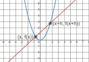

Examples using the Difference Quotient

Compute the difference quotient for the following functions:

a. $f(x)=3x-8$

$\dfrac{f(x+h)-f(x)}{h}$

Evaluate Function: $=\dfrac{3(x+h)-8-(3x-8)}{h}$

Distribute the 3 and the -: $=\dfrac{3x+3h-8-3x+8}{h}$

Cancel 3x-3x and -8+8: $=\dfrac{3h}{h}$

Cancel h’s: $=3$

b. $g(x)=x^2-2x+3$

$\dfrac{f(x+h)-f(x)}{h}$

Evaluate Function: $=\dfrac{(x+h)^2-2(x+h)+3-(x^2-2x+3)}{h}$

Expand the square, distribute the 2 and the -: $=\dfrac{x^2+2xh+h^2-2x-2h+3-x^2+2x-3}{h}$

Cancel x^2’s, 2x and 3’s: $=\dfrac{2xh+h^2-2h}{h}$

Factor out h: $=\dfrac{h(2x+h-2)}{h}$

Cancel h’s: $=2x+h-2$

Warning Triangle with Exclamation Point Be Careful! You have to put (x+h) into the function as one piece and then simply within the function. As a general rule $\color{red}f(x+h)\ne f(x)+f(h)$ You also want to remember to put parentheses around the f(x) because do not want to forget to distribute the negative.

Try it Now 3

a. $f(x)=2x+5$

b. $g(x)=x^2+3x-8$

Application to Business

In business, average rate of change is related to the idea of marginal cost, marginal revenue, and marginal profit.

Marginal Cost/Revenue/Profit

Marginal Cost is typically defined as the change in total cost if the quantity of items produced increases by one. Likewise, marginal revenue and marginal profit are the change in revenue and profit if the quantity of items increases by one.

In practice, marginal cost is usually calculated another way, using calculus techniques you will learn in future courses. In this course, though, we will stick with calculating marginal cost by looking at the actual change of total cost when production increases by one.

Examples

A company has determined the total cost of producing $q$ items is $TC(q)=2000+50\sqrt{q}$ . Find the marginal cost, when production is currently 5000 items.

We want to find the increase in total cost when increasing production from 5000 items to 5001 items. This is equivalent to finding the average rate of change on the interval [5000, 5001].

The total cost at 5000 items is: $TC(5000)=2000+50\sqrt{5000} \approx 5535.53$
The total cost at 5001 items is: $TC(5001)=2000+50 \sqrt{5001} \approx 5535.89$

The marginal cost is $5535.89-5535.53=0.36$ .

To interpret this in words, after producing 5000 items, the additional cost of producing the 5001st item is 36 cents.

Graphical Behavior of Functions

As part of exploring how functions change, it is interesting to explore the graphical behavior of functions.

Increading/Decreasing

A function is increasing on an interval if the function values increase as the inputs increase. Or, as you read left to right, the graph is trending up. More formally, a function is increasing if $f(b)>f(a)$ for any two input values $a$ and $b$ in the interval with $b>a$ . The average rate of change on an increasing function is positive.

A function is decreasing on an interval if the function values decrease as the inputs increase. Or, as you read left to right, the graph is trending down. More formally, a function is decreasing if $f(b)<f(a)$ for any two input values $a$ and $b$ in the interval with $b>a$ . The average rate of change on an increasing function is negative.

Example on Increasing/Decreasing Intervals

Given the function $p(t)$ graphed here, on what intervals does the function appear to be increasing?

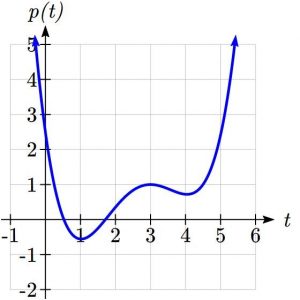
The function appears to be increasing from t = 1 to t = 3, and from t = 4 on.

In interval notation, we would say the function appears to be increasing on the interval $(1,3)$ and the interval $(4,\infty)$ .

Notice that we use open intervals (intervals that don’t include the endpoints) since the function is neither increasing nor decreasing $t=1,3,\,or\,4$ .

Local Extrema

A point where a function changes from increasing to decreasing is called a local maximum.

A point where a function changes from decreasing to increasing is called a local minimum.

Together, local maxima and minima are called the local extrema, or local extreme values, of the function.

Examples of Local Extrema

a. Using the cost of gasoline function from the beginning of the section, find an interval on which the function appears to be decreasing. Estimate any local extrema using the table.

t	2	3	4	5	6	7	8	9
C(t)	1.47	1.69	1.94	2.30	2.51	2.64	3.01	2.14

It appears that the cost of gas increased from $t=2$ to $t=8$ . It appears the cost of gas decreased from $t=8$ to $t=9$ , so the function appears to be decreasing on the interval (8,9).

Since the function appears to change from increasing to decreasing at $t=8$ , there is a local maximum at $t=8$ .

b. Use a graph to estimate the local extrema of the function $f(x)=\dfrac{2}{x}+\dfrac{x}{3}$ .

Use this or your favorite graphing software like Desmos or calculator to determine the intervals on which the function is increasing.

Using technology to graph the function, it appears there is a local minimum somewhere between $x = 2$ and $x =3$ , and a symmetric local maximum somewhere between $x = -3$ and $x = -2$ .

Most graphing calculators and graphing utilities can estimate the location of maxima and minima. Below are screen images from two different technologies, showing the estimate for the local maximum and minimum.

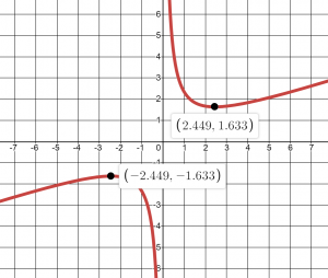
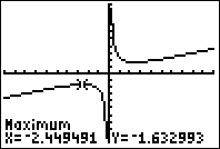
screenshot from Desmos showing both the local minimum and local maximum Screen from TI calculator showing a local maximum point

Based on these estimates, a local maximum occurs at about $(-2.449,-1.633)$ , a local minimum occurs at about $(2.449, 1.633)$ and the function is increasing on the intervals $(-\infty, -2.449)$ and $(2.449, \infty)$ .

Desmos automatically puts a grey dot where the local extrema are which you can click on to display the coordinates, while on a TI-83/84 Calculator, here is a step-by step instruction on doing this. If you need a second set of instructions or have a CASIO, try this instruction page.

Try It Now 4

a. If a company has a total revenue function of $R(x)=15x$ , what would its marginal revenue be when they sell 2000 items?

b. Use a graph of the function $f(x) = {x^3} - 6{x^2} - 15x + 20$ (on Desmos or your calculator) to estimate the local extrema of the function. Use one of these to determine the intervals on which the function is increasing and decreasing.

Try it Now Answers

$\dfrac{{3.01 - 1.69}}{{5 \;years}} = \dfrac{{1.32}}{{5\;years}}=0.264$ dollars per year.

2. a. Average rate of change

$=\dfrac{{f(9) - f(1)}}{{9 - 1}} = \dfrac{{\left( {9 - 2\sqrt 9 } \right) - \left( {1 - 2\sqrt 1 } \right)}}{{9 - 1}} = \dfrac{{\left( 3 \right) - \left( { - 1} \right)}}{{9 - 1}} = \dfrac{4}{8} = \dfrac{1}{2}$

b.

$\dfrac{{f(a + h) - f(a)}}{{(a + h) - a}} = \dfrac{{\left( {{{(a + h)}^2} + 2} \right) - \left( {{a^2} + 2} \right)}}{h} = \dfrac{{{a^2} + 2{a}h + {h^2} + 2 - {a^2} - 2}}{h} = \dfrac{{2{a}h + {h^2}}}{h} = \dfrac{{h\left( {2{a} + {h}} \right)}}{h} = 2{a} + h$

3. a.

$\dfrac{f(x + h) - f(x)}{h} = \dfrac{\left( {2(x + h)} + 5 \right) - \left( {2x} + 5 \right)}{h} = \dfrac{2x + 2h + 5 - 2x - 5}{h} = \dfrac{2h}{h} = 2$

b.

$\dfrac{f(x + h) - f(x)}{h} = \dfrac{\left( (x + h)^2 +3(x+h)-8\right) - \left( x^2 + 3x-8 \right)}{h} = \dfrac{x^2+ 2{x}h + {h^2} + 3x+3h -8 - {x^2} -3x + 8}{h} = \dfrac{2{x}h + 3h+ {h^2}}{h} = \dfrac{h\left( 2x +3+ h \right)}{h} = 2{x} + 3+h$

4. Based on the graph, the local maximum appears to occur at $(-1, 28)$ , and the local minimum occurs at $(5,-80)$ . The function is increasing on $(-\infty,-1) \cup (5,\infty)$ and decreasing on $(-1,5)$ .