7.1 Exponential Functions

Terri Manthey

7.1 Exponential Functions

As this book was being adapted in July 2020, COVID-19, also known as Coronavirus was invading the world. On several dates in June and July, the state of Alaska^[1] had an $R_t$ number of 1.2 and this is with mitigating precautions in place. The $R_t$ is the average number of people that one infected people will, in turn, give it to. For example, if 100 people have it right now, in about a week, 120 people will, or 100 times 1.2. This does not sound like a problem that would cause so much disruption to our daily lives. But consider what happens in a month or two, each of the 120 then, in turn, infect 1.2 others, so the next week, the number is 144, then 172, 207 and these are new case, and often, we have people recovering within a week or two. So for our purposes, we can consider these the current active cases at a time, although it is a low estimate. In three months, the 100 cases turn into over 1000 and in 6 months over 10,000 unless more more mitigating precautions are put into place.

In linear growth, we had a constant rate of change – a constant number that the output increased for each increase in input. For example, in the equation $f(x)=3x+4$ , the slope tells us the output increases by three each time the input increases by one. This population scenario is different – we have a percent rate of change rather than a constant number of people as our rate of change. To see the significance of this difference consider these two companies:
Company A has 100 stores, and expands by opening 50 new stores a year.
Company B has 100 stores, and expands by increasing the number of stores by 50% of their total each year.

Looking at a few years of growth for these companies:

Year	Stores, company A		Stores, company B
0	100	Starting with 100 each	100
1	100 + 50 = 150	They both grow by 50 stores in the first year.	100 + 50% of 100 100 + 0.50(100) = 150
2	150 + 50 = 200	Store A grows by 50, Store B grows by 75	150 + 50% of 150 150 + 0.50(150) = 225
3	200 + 50 = 250	Store A grows by 50, Store B grows by 112.5	225 + 50% of 225 225 + 0.50(225) = 337.5

Notice that with the percent growth, each year the company is grows by 50% of the current year’s total, so as the company grows larger, the number of stores added in a year grows as well.

To try to simplify the calculations, notice that after 1 year the number of stores for company B was:
$100+0.50(100)$
Or equivalently by factoring $100(1+0.50)=100(1.50)=150$

We can think of this as “the new number of stores is the original 100% plus another 50%”.

After 2 years, the number of stores was:
$150 + 0.50(150)$
Or equivalently by factoring $150(1+0.50)=150(1.50)$
Now recall that the 150 came from $100(1.50)$
Substitute that: $100(1.50)(1.50)=100(1.50)^2=225$

After 3 years, the number of stores was:
$225 + 0.50(225)$
Or equivalently by factoring $225(1+0.50)=225(1.50)$
Now recall that the 225 came from $100(1.50)^2$
Substitute that: $100(1.50)^2(1.50)=100(1.50)^3=337.5$

From this, we can generalize, noticing that to show a 50% increase, each year we multiply by a factor of $(1+0.50)$ or $(1.50)$ , so after $n$ years, our equation would be:
$B(n)=100(1+0.50)^n$ or $B(n)=100(1.5)^n$

In this equation, the 100 represented the initial quantity, and the 0.50 was the percent growth rate. Generalizing further, we arrive at the general form of exponential functions.

Exponential Function

An exponential growth or decay function is a function that grows or shrinks at a constant percent growth rate. The equation can be written in the form:

$f(x) = a{(1 + r)^x}$ or equivalently $f(x) = a{b^x}$ where $b=1+r$

Where
$a$ is the initial or starting value of the function
$r$ is the percent growth (if $r>0$ ) or decay (if $r<0$ )
$b$ is a growth factor or growth multiplier. Since powers of negative numbers behave strangely, we limit $b$ to positive values.

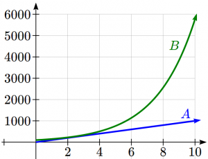
To see more clearly the difference between exponential and linear growth, compare the two tables and graphs below, which illustrate the growth of company A and B described above over a longer time frame if the growth patterns were to continue.

years	Company A	Company B
2	200	225
4	300	506
6	400	1139
8	500	2563
10	600	5767

Graph comparing linear vs exponential growth

Example of an Exponential Function

Write an exponential function for the spread of COVID-19 when the R-number is $R_t=1.2$ and predict how many cases would be active 15 weeks after 100 cases are active.

We are given, $b$ in this case, the growth factor. Our $R_t=b$ so we will use the function $f(t)=ab^t$ If we were using the other function, we could recognize that $b=r+1$ so our percent growth rate would be 0.2 or 20%. When the R numbers is 1.2, the coronavirus active cases is growing by 20% per week. We are starting at 100 cases so:

Our formula becomes $f(t)=100(1.2)^t$

To estimate the number of cases in 15 weeks assuming the R number stays constant, we plug in 15 for $t$ .

$f(15)=100(1.2)^15 \approx 1541$ active cases 15 weeks from now.

Remember the total number of cases would be much higher, because you would have to consider the ones that were already counted.

Try it Now 1

Given the three statements below, identify which represent exponential functions.

A. The cost of living allowance for state employees is $1250 right now and increases by 3.1% each year.
B. State employees can expect a $300 raise each year they work for the state.
C. Tuition costs have increased by 2.8% each year for the last 3 years.

For the first exponential function, write the function that would show what the result would be after t years.

Example of a Financial Applications

A certificate of deposit (CD) is a type of savings account offered by banks, typically offering a higher interest rate in return for a fixed length of time you will leave your money invested. If a bank offers a 24 month CD with an annual interest rate of 1.2% compounded monthly, how much will a $1000 investment grow to over those 24 months?

First, we must notice that the interest rate is an annual rate, but is compounded monthly, meaning interest is calculated and added to the account monthly.

To find the monthly interest rate, we divide the annual rate of 1.2% by 12 since there are 12 months in a year: 1.2%/12 = 0.1%. Each month we will earn 0.1% interest. From this, we can set up an exponential function, with our initial amount of $1000 and a growth rate of r = 0.001, and our input m measured in months.

$f(m) = 1000{\left( {1 + \frac{{.012}}{{12}}} \right)^m}$

$f(m) = 1000{(1 + 0.001)^m}$

After 24 months, the account will have grown to $f(24) = 1000{(1 + 0.001)^{24}} =$ $ 1024.28

Try it Now 2

Looking at these two equations that represent the balance in two different savings accounts, which account is growing faster, and which account will have a higher balance after 3 years?

$A(t) = 1000{\left( {1.05} \right)^t}$ $B(t) = 900{\left( {1.075} \right)^t}$

In all the preceding examples, we saw exponential growth. Exponential functions can also be used to model quantities that are decreasing at a constant percent rate. An example of this is radioactive decay, a process in which radioactive isotopes of certain atoms transform to an atom of a different type, causing a percentage decrease of the original material over time.

Example of Exponential Decay

Bismuth-210 is an isotope that radioactively decays by about 13% each day, meaning 13% of the remaining Bismuth-210 transforms into another atom (polonium-210 in this case) each day. If you begin with 100 mg of Bismuth-210, how much remains after one week?

With radioactive decay, instead of the quantity increasing at a percent rate, the quantity is decreasing at a percent rate. Our initial quantity is a = 100 mg, and our growth rate will be negative 13%, since we are decreasing: r = -0.13. This gives the equation:
$Q(d)=100(1-0.13)^d=100(0.87)^d$
This can also be explained by recognizing that if 13% decays, then 87% remains.

After one week, 7 days, the quantity remaining would be
$Q(7)=100(0.87)^7=37.73$ mg of Bismuth-210 remains.

Try it Now 3

Vermont’s Coronavirus cases have a low R number. Their new cases are slowing by a rate of 12% per week^[2]. If they currently have 160 active cases^[3] If the cases keep declining at this rate, how many active cases is Vermont expected to have in 6 weeks?

Example Interpret an Exponential Function Equation

$T(q)$ represents the total number of Android smart phone contracts, in thousands, held by a certain Verizon store region measured quarterly (every 3 months) since January 1, 2010.
Interpret all of the parts of the equation $T(2) = 86{(1.64)^2} = 231.3056$

Interpreting this from the basic exponential form, we know that 86 is our initial value. This means that on Jan. 1, 2010 this region had 86,000 Android smart phone contracts. Since b = 1 + r = 1.64, we know that every quarter the number of smart phone contracts grows by 64%. $T(2) = 231.3056$ means that in the 2nd quarter (or at the end of the second quarter) there were approximately 231,305 Android smart phone contracts.

Finding Equations of Exponential Functions

In the previous examples, we were able to write equations for exponential functions since we knew the initial quantity and the growth rate. If we do not know the growth rate, but instead know only some input and output pairs of values, we can still construct an exponential function.

Example Finding a Formula for an Exponential Function

In 2012, a company had 80 retail stores. By 2018, the company had grown to 180 retail stores. If the company is growing exponentially, find a formula for the function.

By defining our input variable to be t, years after 2012, the information listed can be written as two input-output pairs: (0,80) and (6,180). Notice that by choosing our input variable to be measured as years after the first year value provided, we have effectively “given” ourselves the initial value for the function: $a = 80$ . This gives us an equation of the form
$f(t)=80b^t$

Substituting in our second input-output pair allows us to solve for b:
$180=80b^6$
$b^6=\dfrac{180}{80}=\dfrac{9}{4}$
Now take the 6th root of both sides (with a calculator, you can either use the ^ key or $y^x$ key with $\frac{1}{6}$ or on a TI, type in the 6 and hit MATH 5 and then the inside of the root.)
$b=\sqrt[6]{\dfrac{9}{4}}\approx 1.1447$

This gives us our equation for the population:
$f(t)=80(1.447)^t$

Recall that since $b = 1+r$ , we can interpret this to mean that the population growth rate is $r = 0.1447$ , and so the population is growing by about 14.47% each year.

In the above example, we chose to use the $f(x)=ab^x$ form of the exponential function rather than the $f(x)=a(1+r)^x$ form, but this choice was entirely arbitrary – either form would be fine to use.

When finding equations, the value for b or r will usually have to be rounded to be written easily. To preserve accuracy, it is important to not over-round these values. Typically, you want to be sure to preserve at least 3 significant digits in the growth rate. For example, if your value for b was 1.00317643, you would want to round this no further than to 1.00318.

Try it Now 4

Find the formula for an exponential passing through (0, 10) and (3, 7).

Graphs of Exponentials

To get a sense for the behavior of exponentials, let us begin by looking more closely at the function $f(x)=2^x$ . Listing a table of values for this function:

x	-3	-2	-1	0	1	2	3
f(x)	$\frac{1}{8}$	$\frac{1}{4}$	$\frac{1}{2}$	1	2	4	8

Notice that:

This function is positive for all values of $x$ .
As $x$ increases, the function grows faster and faster (the rate of change increases).
As $x$ decreases, the function values grow smaller, approaching zero.
This is an example of exponential growth.

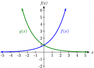
Looking at the function $g(x)=\left(\dfrac{1}{2}\right)^x$

x	-3	-2	-1	0	1	2	3
g(x)	8	4	2	1	$\frac{1}{2}$	$\frac{1}{4}$	$\frac{1}{8}$

Note this function is also positive for all values of x, but in this case grows as x decreases, and decreases towards zero as x increases. This is an example of exponential decay. You may notice from the table that this function appears to be the horizontal reflection of the $f(x)=2^x$ table. This is in fact the case:
$f(-x)=2^-x=\left(2^-1\right)^x=\left(\dfrac{1}{2}\right)^x=g(x)$

Looking at the graphs also confirms this relationship:

Graphs of 2^x and (1/2)^x on same graph

Consider a function for the form $f(x)=ab^x$ . Since a, which we called the initial value in the last section, is the function value at an input of zero, a will give us the vertical intercept of the graph. From the graphs above, we can see that an exponential graph will have a horizontal asymptote on one side of the graph, and can either increase or decrease, depending upon the growth factor. This horizontal asymptote will also help us determine the long run behavior and is easy to determine from the graph.

The graph will grow when the growth rate is positive, which will make the growth factor b larger than one. When it’s negative, the growth factor will be less than one.

Graphical Features of Exponential Functions

Graphically, in the function $f(x)=ab^x$

$a$ is the vertical intercept of the graph
determines the rate at which the graph grows. What is postive:
- the function will increase if $b>1$
- the function will decrease if $0<b<1$
The graph will have a horizontal asymptote at $y=0$
The graph will be concave up if $a>0$ and concave down if $a<0$
The domain of the function is all real numbers
The range of the function is $(0,\infty)$

When sketching the graph of an exponential function, it can be helpful to remember that the graph will pass through the points $(0, a)$ and $(1, ab)$ .

The value $b$ will determine the function’s long run behavior:
If $b>1$ , as $x \to \infty,\;f(x) \to \infty$ and as $x \to -\infty,\;f(x) \to 0$ .
If $0<b<1$ , as $x \to \infty,\;f(x) \to 0$ and as $x \to -\infty,\;f(x) \to \infty$ .

Example Graphing a Function of the form $\color{white} y=ab^x$

Sketch a graph of $f(x) = 4{\left( {\dfrac{1}{3}} \right)^x}$

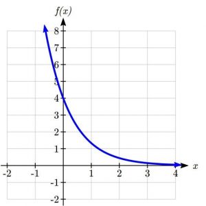
This graph will have a vertical intercept at (0,4), and pass through the point $\left(1, \dfrac{4}{3}\right)$ . Since $b<1$ , the graph will be decreasing towards zero. Since $a>0$ , the graph will be concave up.

We can also see from the graph the long run behavior: as $x \to \infty,\;f(x) \to 0$ and as $x \to -\infty,\;f(x) \to \infty$ .

To get a better feeling for the effect of a and b on the graph, examine the sets of graphs below. The first set shows various graphs, where a remains the same and we only change the value for b.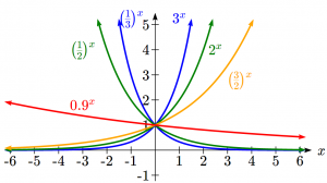 Graph of various exponential functions with different base b

Notice that the closer the value of b is to 1, the less steep the graph will be.

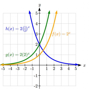
In the next set of graphs, a is altered and our value for b remains the same.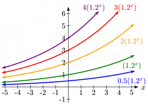 Graph of Various Exponential Functions with Base 1.2 and different initial values a

Notice that changing the value for a changes the vertical intercept. Since a is multiplying the bx term, a acts as a vertical stretch factor, not as a shift. Notice also that the long run behavior for all of these functions is the same because the growth factor did not change and none of these a values introduced a vertical flip.

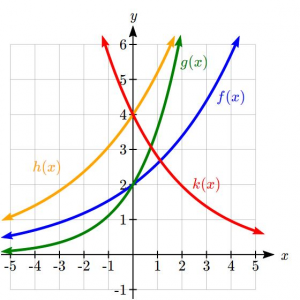
Example Identifying Graphs of Exponential Functions

Match each equation with its graph.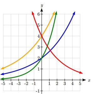

$\begin{array}{l} f(x) = 2{(1.3)^x}\\ g(x) = 2{(1.8)^x}\\ h(x) = 4{(1.3)^x}\\ k(x) = 4{(0.7)^x} \end{array}$

The graph of k(x) is the easiest to identify, since it is the only equation with a growth factor less than one, which will produce a decreasing graph. The graph of h(x) can be identified as the only growing exponential function with a vertical intercept at (0,4). The graphs of f(x) and g(x) both have a vertical intercept at (0,2), but since g(x) has a larger growth factor, we can identify it as the graph increasing faster.

Example Graphs for this problem labeled with the correct functions

Try it Now 5

Graph the following functions on the same axis: $f(x)=2^x; \;g(x)=2(2)^x; \;h(x)=2\left(\dfrac{1}{2}\right)^x$

Compound Interest

In the bank certificate of deposit (CD) example earlier in the section, we encountered compound interest. Typically bank accounts and other savings instruments in which earnings are reinvested, such as mutual funds and retirement accounts, utilize compound interest. The term compounding comes from the behavior that interest is earned not on the original value, but on the accumulated value of the account. We’ll explore compound interest in greater depth in a later chapter, but will introduce basics here.

In the example from earlier, the interest was compounded monthly, so we took the annual interest rate, usually called the nominal rate or annual percentage rate (APR) and divided by 12, the number of compounds in a year, to find the monthly interest. The exponent was then measured in months.

Generalizing this, we can form a general formula for compound interest. If the APR is written in decimal form as $r$ , and there are $k$ compounding periods per year, then the interest per compounding period will be $\dfrac{r}{k}$ . Likewise, if we interested in the value after $t$ years, then there will be $kt$ compounding periods in that time.

Compound Interest Formula

Compound Interest can be calculated using the formula

$A(t) = a{\left( {1 + \frac{r}{k}} \right)^{kt}}$

Where

$A(t)$ is the account value
$t$ is measured in years
$a$ is the starting amount of the account, often called principal
$r$ in the annual percentage rate (APR), also called the nominal rate
$k$ is the number of compounding periods in one year

Examples of Compound Interest

a. If you invest $3,000 in an investment account paying 3% interest compounded quarterly, how much will the account be worth in 10 years?

Since we are starting with $3000, a = 3000
Our interest rate is 3%, so r = 0.03
Since we are compounding quarterly, we are compounding 4 times per year, so k = 4
We want to know the value of the account in 10 years, so we are looking for A(10), the value when t = 10.

$A(10) = 3000{\left( {1 + \frac{{0.03}}{4}} \right)^{4(10)}} = $ 4045.05$

The account will be worth $4045.05 in 10 years

b. A 529 plan is a college savings plan in which a relative can invest money to pay for a child’s later college tuition, and the account grows tax free. If Nuru wants to set up a 529 account for her new granddaughter, wants the account to grow to $40,000 over 18 years, and she believes the account will earn 6% compounded semi-annually (twice a year), how much will Nuru need to invest in the account now?

Since the account is earning 6%, $r = 0.06$
Since interest is compounded twice a year, $k = 2$

In this problem, we don’t know how much we are starting with, so we will be solving for $a$ , the initial amount needed. We do know we want the end amount to be $40,000, so we will be looking for the value of a so that A(18) = 40,000.

$\begin{array}{l} 40,000 = A(18) = a{\left( {1 + \frac{{0.06}}{2}} \right)^{2(18)}}\\ /;\\ 40,000 = a(2.8983)\\ \;\\ a = \dfrac{{40,000}}{{2.8983}} \approx $ 13,801 \end{array}$

Nuru will need to invest $13,801 to have $40,000 in 18 years.

Try it Now 6

If you invest $3,000 in an investment account paying 3% interest compounded monthly how much will the account be worth in 10 years?

A Limit to Compounding

Because of compounding throughout the year, with compound interest the actual increase in a year is more than the annual percentage rate. If $1,000 were invested at 10%, the table below shows the value after 1 year at different compounding frequencies:

Frequency	Value after 1 year
Annually	$1100
Semiannually	$1102.50
Quarterly	$1103.81
Monthly	$1104.71
Daily	$1105.16

The amount we earn increases as we increase the compounding frequency. Notice, though, that the increase from annual to semi-annual compounding is larger than the increase from monthly to daily compounding. This might lead us to believe that although increasing the frequency of compounding will increase our result, there is an upper limit to this process.

To see this, let us examine the value of $1 invested at 100% interest for 1 year.

Frequency	Value
Annual	$2
Semiannually	$2.25
Quarterly	$2.441406
Monthly	$2.613035
Daily	$2.714567
Hourly	$2.718127
Once per minute	$2.718279
Once per second	$2.718282

These values do indeed appear to be approaching an upper limit. This value ends up being so important that it gets represented by its own letter, much like how $\pi$ represents a number.

Euler’s Number: e

e is the letter used to represent the value that ${\left( {1 + \frac{1}{k}} \right)^k}$ approaches as $k$ gets big.

$e \approx 2.719282$

Because e is often used as the base of an exponential, most scientific and graphing calculators have a button that can calculate powers of e, usually labeled $e^x$ . Some computer software instead defines a function $exp(x)$ , where $exp(x)=e^x$

Because e arises when the time between compounds becomes very small, e allows us to define continuous growth and allows us to define a new toolkit function, $f(x)=e^x$ .

Continuous Growth Formula

Continuous Growth can be calculated using the formula

$f(x)=ae^{rx}$

where

$a$ is the starting amount
$r$ is the continuous growth rate

This type of equation is commonly used when describing quantities that change more or less continuously, like chemical reactions, growth of large populations, and radioactive decay. It is also used extensively in calculus.

Example of Continuous Decay

Radon-222 decays at a continuous rate of 17.3% per day. How much will 100mg of Radon-222 decay to in 3 days?

Since we are given a continuous decay rate, we use the continuous growth formula. Since the substance is decaying, we know the growth rate will be negative: $r = -0.173$
$f(3)=100e^{-0.173(3)} \approx 59.512$ mg of Radon-222 will remain.

Try it Now 7

Interpret the following: $S(t)=20e^{0.12t}$ if $S(t)$ represents the growth of a substance in grams, and time is measured in days.

Continuous growth is also often applied to compound interest, allowing us to talk about continuous compounding.

Example of Continuous Compounding

If $1000 is invested in an account earning 10% compounded continuously, find the value after 1 year.

Here, the continuous growth rate is 10%, so $r = 0.10$ . We start with $1000, so $a = 1000$ .
To find the value after 1 year,
$f(1) = 1000{e^{0.10(1)}} \approx $ 1105.17$

Notice this is a $105.17 increase for the year. As a percent increase, this is
$\frac{{105.17}}{{1000}} = 0.10517 = 10.517\%$ increase over the original $1000.

Notice that this value is slightly larger than the amount generated by daily compounding in the table computed earlier.

The continuous growth rate is like the nominal growth rate (or APR) – it reflects the growth rate before compounding takes effect. This is different than the annual growth rate used in the formula $f(x) = a{(1 + r)^x}$ , which is like the annual percentage yield (APY, also called the effective rate) – it reflects the actual amount the output grows in a year.

While the continuous growth rate in the example above was 10%, the actual annual yield was 10.517%. This means we could write two different looking but equivalent formulas for this account’s growth:
$f(t) = 1000{e^{0.10t}}$ using the 10% continuous growth rate
$f(t) = 1000(1.10517)^t$ using the 10.517% actual annual yield rate

Try it Now Answers

. A & C are exponential functions, they grow by a % not a constant number. $f(t)=1250(1.031)^t$
$B(t)$ is growing faster, but after 3 years $A(t)$ still has a higher account balance.
$f(t)=160(0.88)^t; \; f(6) \approx 74$ people
$f(x) = 10{(0.8879)^x}$
$4048.06
An initial substance weighing 20g is growing at a continuous rate of 12% per day.