2.6 Modeling with Linear Functions

Terri Manthey

2.6 Modeling with Linear Functions

When modeling scenarios with a linear function and solving problems involving quantities changing linearly, we typically follow the same problem solving strategies that we would use for any type of function:

Problem Solving Strategies

1. Identify changing quantities, and then carefully and clearly define descriptive variables to represent those quantities. When appropriate, sketch a picture or define a coordinate system.

2. Carefully read the problem to identify important information. Look for information giving values for the variables, or values for parts of the functional model, like slope and initial value.

3. Carefully read the problem to identify what we are trying to find, identify, solve, or interpret.

4. Identify a solution pathway from the provided information to what we are trying to find. Often this will involve checking and tracking units, building a table or even finding a formula for the function being used to model the problem.

5. When needed, find a formula for the function.

6. Solve or evaluate using the formula you found for the desired quantities.

7. Reflect on whether your answer is reasonable for the given situation and whether it makes sense mathematically.

8. Clearly convey your result using appropriate units, and answer in full sentences when appropriate.

Examples Modeling with Linear Functions

a. A company purchased $120,000 in new office equipment. Then expect the value to depreciate (decrease) by $16,000 per year. Find a linear model for the value, then find and interpret the horizontal intercept and determine a reasonable domain and range for this function.

In the problem, there are two changing quantities: time and value. The remaining value of the equipment depends on how long the company has had it. We can define our variables, including units.

Output: V, value remaining, in dollars

Input: t, time, in years

Reading the problem, we identify two important values. The first, $120,000, is the initial value for V. The other value appears to be a rate of change – the units of dollars per year match the units of our output variable divided by our input variable. The value is depreciating, so you should recognize that the value remaining is decreasing each year and the slope is negative.

Using the intercept and slope provided in the problem, we can write the equation: $V(t)=120,000-16,000t$

To find the horizontal intercept, we set the output to zero, and solve for the input:
$0=120000-16000t$
$t=\dfrac{120,000}{16,000}=7.5$

The horizontal intercept is 7.5 years. Since this represents the input value where the output will be zero, interpreting this, we could say: The equipment will have no remaining value after 7.5 years.

When modeling any real life scenario with functions, there is typically a limited domain over which that model will be valid – almost no trend continues indefinitely. In this case, it certainly doesn’t make sense to talk about input values less than zero. This model is also not valid after the horizontal intercept.

The domain represents the set of input values and so the reasonable domain for this function is $0 \leq t \leq 7.5$ . The range represents the set of output values and the value starts at $120,000 and ends with $0 after 7.5 years so the corresponding range is $0 \leq V(t) \leq 120,000$ .

Most importantly remember that domain and range are tied together, and what ever you decide is most appropriate for the domain (the independent variable) will dictate the requirements for the range (the dependent variable).

b. Jamal is choosing between two moving companies. The first, U-Haul, charges an up-front fee of $29.95, then 79 cents a mile. The second, Ryder, charges an up-front fee of $106.95, then 19 cents a mile^[1]. How many miles will Jamal have to drive in order for Ryder to be a better deal than U-haul?

The two important quantities in this problem are the cost, and the number of miles that are driven. Since we have two companies to consider, we will define two functions:

Input: m, miles driven
Outputs:
$U(m)$ : cost, in dollars, for renting from U-haul
$R(m)$ : cost, in dollars, for renting from Ryder

Reading the problem carefully, it appears that we were given an initial cost and a rate of change for each company. Since our outputs are measured in dollars but the costs per mile given in the problem are in cents, we will need to convert these quantities to match our desired units: $0.79 a mile for U-Haul and $0.19 a mile for Ryder.

Looking to what we’re trying to find, we want to know when Ryder will be the better choice. Since all we have to make that decision from is the costs, we are looking for when Ryder will cost less, or when $R(m)<U(m)$ . The solution pathway will lead us to find the equations for the two functions, find the intersection, then look to see where the Y(m) function is smaller. Using the rates of change and initial charges, we can write the equations:
$U(m)=29.95+0.79m$
Graph showing the cost of uhaul vs cost of ryder tuck $R(m)=106.95+0.19m$

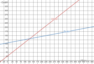
These graphs are sketched to the right.

To find the intersection, we set the equations equal and solve: $U(m)=R(m)$

$29.95+0.79m=106.95+0.19m$
$0.6m=77$
$m=128.33$

This tells us that at 128.3 miles, the cost from the two companies will be about the same. Either by looking at the graph, or noting that $R(m)$ is growing at a slower rate, we can conclude that Ryder will be the cheaper price when 183 or more miles are driven, but for 182 or fewer miles driven, the cheaper cost would be from U-haul.

Note: You could also look at the Desmos graph or use the Intersection feature on the your calculator to find this point as well.

c. A company’s revenue has been growing linearly. In 2015, their revenue was $1.45 million. By 2018, the revenue had grown to $1.81 million. If this trend continues (Let’s say this is a company in an industry which was not overly affected by the COVID-19 Pandemic.)

i. Predict the revenue in 2023
ii. When will the revenue reach $3 million?

The two changing quantities are the revenue and time. While we could use the actual year value as the input quantity, doing so tends to lead to very ugly equations, since the vertical intercept would correspond to the year 0, more than 2000 years ago!

To make things a little nicer, and to make our lives easier too, we will define our input as years since 2015:
Input: t years since 2015
Output: $R(t)$ , the company’s revenue, in millions of dollars

The problem gives us two input-output pairs. Converting them to match our defined variables, the year 2015 would correspond to $t = 0$ , giving the point (0, 1.45). Notice that through our clever choice of variable definition, we have “given” ourselves the vertical intercept of the function. The year 2018 would correspond to $t = 3$ , giving the point (3, 1.81).

To predict the population in 2023 ( $t = 8$ ), we would need an equation for the population. Likewise, to find when the revenue would reach $3 million, we would need to solve for the input that would provide an output of 3. Either way, we need an equation. To find it, we start by calculating the rate of change:
$m=\dfrac{1.81-1.45}{3-0}=\dfrac{0.36}{3}=0.12$ million dollars per year.

Since we already know the vertical intercept of the line, we can immediately write the equation:
$R(t)=1.45+.12t$

To predict the revenue in 2023, we evaluate our function at $t=8$
$R(8)=1.45+0.12(8)=2.41$
If the trend continues, our model predicts a revenue of $2.41 million in 2023.

To find when the population will reach $3 million, we can set $R(t)=3$ and solve for $t$ :
$3=1.45+0.12t$
$1.55=0.12t$
$t=12.917$

Our model predicts the revenue will reach $3 million in a little under 13 years after 2015, or just before the year 2028.

Modelling Cost, Revenue and Profit

In business, a very common application of functions is to model cost, revenue, and profit.

Cost, Revenue and Profit

When a company produces q items, the total cost is the cost of total cost of producing those items. The total cost includes both fixed costs, which are startup costs, like equipment and buildings, and variable costs, which are costs that depend on the number of items produced, like materials and labor.

In the most simple case, Total Cost = (Fixed Costs) + (Variable Costs) ∙ q

Revenue is the amount of money a company brings in from sales.

In the most simple case, Revenue = (Revenue per item) ∙ q

Profit is the amount of money brings in, after expenses.

Profit = Revenue – Costs

We often talk about the break-even point. This is the level of production where Revenue equals Cost, or equivalently where Profit is zero. This is typically the minimum level of sales necessary for the company to make a profit.

Example Examining Cost, Revenue and Profit

A tech startup is looking at developing and launching a new mobile app. Initial development of the app will cost $300,000, and they estimate marketing and support for each user will cost $0.50. While the app will be free, they estimate they will be able to bring in $2 per user on average from in-app purchases. How many users will the company need to break even?

We start by modeling the cost, revenue, and profit. Let x = number of users.

The fixed (initial) costs are $300,000, and the variable (per-item) costs as $0.50 per user. We can write the total cost equation:
$C(x)=300,000+0.50x$

The revenue will be $2 per user, so the revenue equation will be:
$R(x)=2x$

We could find the break-even point by setting the total cost equal to the revenue, which is equivalent to finding the intersection of the lines.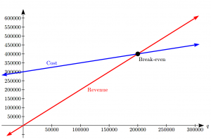

Alternatively, we could go ahead and find a profit equation first:
$P(x)=R(x)-C(x)=2x-(300,000+0.5x)=1.5x-300,000$

The break even point can be found by setting the profit equal to zero:
$0=1.5x-300,000$
$1.5x=300,000$
$x=200,000$

The company will have to acquire 200,000 users to break even.

Try it Now 1

A donut shop estimates their fixed daily expenses are $600. If each donut costs about $0.05 to make and sells for $0.60, how many donuts do they need to sell to break even?

Supply and Demand

In economics, there is a model for how prices are determined in a free market which states that supply and demand for a product is related to the price. The demand relationship shows the quantity of a certain product that consumers are willing to buy at a certain price. Typically the quantity demanded will decrease for an item if the price increases. The supply relationship shows the quantity of a product that suppliers are willing to produce at a certain sales price. Typically the supply demanded will increase if the price increases. Economic theory says that supply and demand will interact, and the intersection will be the equilibrium price, or market price, where the quantity supplied and demanded will be equal.

Supply and Demand

If $p$ is the price of a product, then
$Q_d$ is the quantity demanded.
$Q_s$ is the quantity supplied.

The demand curve is a decreasing function while the supply curve in an increasing function.

The intersection of the curves is the equilibrium price and quantity, also called the market price and quantity. This point is often notated as $p^*, Q^*$ .

In later chapters you will explore supply and demand curves that are non-linear, but in this chapter we will focus on linear supply and demand functions.

In most economic books, you will see the supply and demand curve written with price as the input and quantity as the output, like $Q_d=140-2p$ . However, supply and demand graphs are drawn with price on the vertical axis and quantity on the horizontal. In an effort to avoid confusion, most of the time in this text we will instead write supply and demand curves with price as the output, to match its placement on the vertical axis.

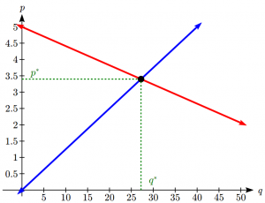
Example of Supply and Demand

At a price of $2.50 per gallon, there is a demand in a certain town for 42.5 thousand gallons of gas and a supply of 20 thousand gallons. At a price of $3.50, there is demand for 25.5 thousand gallons and a supply of 28 thousand gallons. Assuming supply and demand are linear, find the equilibrium price and quantity.

We start by finding a linear equation for both supply and demand. We will use price, p in dollars, as the output and quantity, q in thousands of gallons, as the input.

For supply, we have the points (20, 2.50) and (28, 3.50).

Finding the slope: $m=\dfrac{3.50-2.50}{28-20}=\dfrac{1}{8}$

We know the equation will look like $p=\dfrac{1}{8}q+b$ , so substituting in (20, 2.50),
$2.5=\dfrac{1}{8}(20)+b$
$2.5=2.5+b$
$b=0$

The supply equation is: $p=\dfrac{1}{8}q$

For demand, we have the points (42.5, 2.50) and (25.5, 3.50).

Finding the slope: $m=\dfrac{3.50-2.50}{25.5-42.5}=\dfrac{1}{-17}$

We know the equation will look like $p=-\dfrac{1}{17}q+b$ , so substituting in (42.5, 2.50),
$2.5=-\dfrac{1}{17}(42.5)+b$
$2.5=-2.5+b$
$b=5$

The demand equation is: $p=-\dfrac{1}{17}q+5$

To find the equilibrium, we set the supply equal to the demand:
$\dfrac{1}{8}q=-\dfrac{1}{17}q+5$
Multiply through by 8(17) = 136 to clear the fractions:
$136 \left(\dfrac{1}{8}q \right)=136 \left(-\dfrac{1}{17}q+5 \right)$
$17q=-8q+680$
Now we solve for $q$ :
$25q=680$
$q=27.2$

To find the equilibrium price, we can substitute that value back into either equation: $p=\dfrac{1}{8}(27.2)=3.4$

The equilibrium quantity will be 27.2 thousand gallons of gas at a price of $3.40.

Supply and Demand Graph

Try it Now 2

A company estimates that at a price of $140 there will demand for 4000 items, and for each $5 increase in price the demand will drop by 200 items. The supply curve is $p=\dfrac{1}{20}q$ . Find the equilibrium price and quantity.