4.2 Graphical Solutions of Linear Programming

Terri Manthey

4.2 Graphical Solutions of Linear Programming

Wouldn’t it be nice if we could simply produce and sell infinitely many units of a product and thus make a never-ending amount of money? In business (and in day-to-day living) we know that some things are just unreasonable or impossible. Instead, our hope is to maximize or minimize some quantity, given a set of constraints.

In order to have a linear programming problem, we must have:

Constraints, represented as inequalities
An objective function, which is a function whose value we either want to be a large as possible (want to maximize it) or as small as possible (want to minimize it).

Let’s consider an extension of the example from the end of the last section:

Example of Linear Programming

A company produces a basic and premium version of its product. The basic version requires 20 minutes of assembly and 15 minutes of painting. The premium version requires 30 minutes of assembly and 30 minutes of painting. If the company has staffing for 3,900 minutes of assembly and 3,300 minutes of painting each week. They sell the basic products for a profit of $30 and the premium products for a profit of $40. How many of each version should be produced to maximize profit?

Let b = the number of basic products made, and p = the number of premium products made. Our objective function is what we’re trying to maximize or minimize. In this case, we’re trying to maximize profit. The total profit, P, is:
$P=30b+40p$

In the last section, the example developed our constraints. Together, these define our linear programming problem:

Objective function: MAX $P=30b+40p$
Constraints: (We often say “Subject to:” or for short s.t.)
$\begin{array}{l} 20b+30p \leq 3900\\ 15b+30p \leq 3300\\ b \geq 0, p \geq 0 \end{array}$

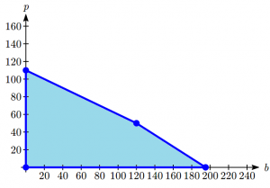
In this section, we will approach this type of problem graphically. We start by graphing the constraints to determine the feasible region – the set of possible solutions. Just showing the solution set where the four inequalities overlap, we see a clear region.

Feasible Region for Example Solution set of constraint inequalities

To consider how the objective function connects, suppose we considered all the possible production combinations that gave a profit of P = $3000, so that $3000=30b+40p$ .That set of combinations would form a line in the graph. Doing the same for a profit of $5000 and $6500 would give additional lines. Graphing those on top of our feasible region, we see a pattern:

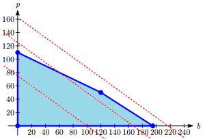
Feasible Region with possible profit lines on top

Notice that all the constant-profit lines are parallel, and that in general the profit increases as we move up to upper right. Notice also that for a profit of $5000 there are some production levels inside the feasible region for that profit level, but some are outside. That means we could feasibly make $5000 profit by producing, for example, 167 basic items and no premium items, but we can’t make $5000 by producing 125 premium items and no basic items because that falls outside our constraints.

The solution to our linear programming problem will be the largest possible profit that is still feasible. Graphically, that means the line furthest to the upper-right that still touches the feasible region on at least point. That solution is the one below:

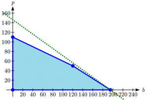
Feasible Region with Highest Profit Function Line

This profit line touches the feasible region where $b = 195$ and $p = 0$ , giving a profit of $P=30(195)+40(0)=5850$ .

Notice that this is slightly larger than the profit that would be made by completely utilizing all staffing at $b = 120$ , $p = 50$ , where the profit would be $5600 or at $b=0$ , $p=110$ , which would be $4400$ and definitely better that (0,0) because that would be $0.

The objective function along with the four corner points above forms a bounded linear programming problem. That is, imagine you are looking at three fence posts connected by fencing (black point and lines, respectively). If you were to put your dog in the middle, you could be sure it would not escape (assuming the fence is tall enough). If this is the case, then you have a bounded linear programming problem. If the dog could walk infinitely in any one direction, then the problem is unbounded.

In the past example, you can see that the line of maximum profit will always touch the boundary of the feasible region. That observation inspires the fundamental theorem of linear programming.

Fundamental Theorem of Linear Programming

If a solution exists to a bounded linear programming problem, then it occurs at one of the corner points.
If a feasible region is unbounded, then a maximum value for the objective function does not exist.
If a feasible region is unbounded, and the objective function has only positive coefficients, then a minimum value exists.

In the last example we solve the problem somewhat intuitively by “sliding” the profit line up. Typically we use a more procedural approach.

Solving a Linear Programming Problem Graphically

Define the variables
Define the variable to be optimized. The question asked is a good indicator as to what this will be: Profit, Revenue, Cost are popular choices.
Write the objective function, as a mathematical equation, like P=10x+15y or C=200a+300b.
Write the constraints as a system of mathematical inequalities
Graph the constraint system of inequalities and shade the feasible region
Identify the corner point by solving systems of linear equation whose intersection represents a corner point.
Test each corner point in the objective function. The “winning” point is the point that optimizes the objective function (greatest if maximizing, least if minimizing.)

Take Note Note that if there is a tie for the winning point in that two points are the max or min, then the objective function is optimized at any point along the line connecting them.

Try it Now 1

Maximize $P=14x+9y$ subject to the constraints:

$\begin{array}{l} x+y \leq 9\\ 3x + y \leq 15\\ x \geq 0, y \geq 0 \end{array}$

Another Linear Programming Example

A health-food business would like to create a high-potassium blend of dried fruit in the form of a box of 10 fruit bars. It decides to use dried apricots, which have 407 mg of potassium per serving, and dried dates, which have 271 mg of potassium per serving. The company can purchase its fruit through in bulk for a reasonable price. Dried apricots cost $9.99/lb. (about 3 servings) and dried dates cost $7.99/lb. (about 4 servings). The company would like the box of bars to have at least the recommended daily potassium intake of about 4700 mg, and contain at least 1 serving of each fruit. In order to minimize cost, how many servings of each dried fruit should go into the box of bars?

Step 1: Define the variables.
$x=$ number of servings of dried apricots
$y=$ number of servings of dried dates

Step 2: We next work on the objective function.

For apricots, there are 3 servings per pound. So the cost per serving is $9.99/3 =$3.33. The cost for $x$ servings would thus by 3.33x

For dates, there are 4 servings per pound. This means the cost per serving is $7.99/4=$2.00. The cost for $y$ servings would thus be 2y.

Step 4: The total cost, $C$ , for apricots and dates would be
$C=3.33x+2y$

Step 4: Normally we would have constraints $x \geq 0$ and $y \geq 0$ since negative servings can’t be used. But in this case, we’re further restricted. In words:

There just be at least 1 serving of each fruit
The product must contain at least 4700 mg of potassium

Mathematically,

Since there must be at least 1 serving of each fruit, then $x \geq 1, y \geq 1$
There are $407x$ mg of potassium in $x$ servings of apricots and $271y$ mg of potassium in $y$ servings of dates. The sum should be greater than or equal to 4700mg of potassium, or $407x+271y \geq 4700$

Thus, we have,

Objective function: MIN $C=3.33x+2y$

Subject to:

$\begin{array}{l} 407x+271y \geq 4700\\ x \geq 1\\ y \geq 1 \end{array}$

Step 5: We graph the constraints and shade the feasible region:

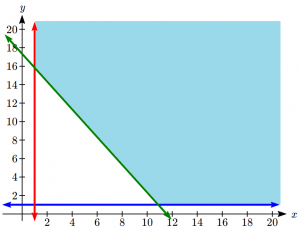
Graph for the fruit Linear programming example

Step 6: The region is unbounded, but we will be able to find a minimum still. We can see there are two corner points.

The one in the upper left is the intersection of the lines $407x+271y=4700$ and $<em>x</em> = 1$ . Solving for the intersection using substitution:
$407(1)+271y=4700$
$y \approx 15.8$
Point: (1, 15.8)

The one in the lower right is the intersection of the lines $407x+271y=4700$ and $y=1$ .
$407x+271(1)=4700$
$x \approx 10.9$
Point: (10.9,1)

Step 7: Testing the objective function at each of these corner points:

Point

Cost, C = 3.33x + 2.00y

(10.9, 1)

C = 3.33(10.9) + 2.00(1) = $38.30

(1, 15.8)

C = 3.33(1) + 2.00(15.8) = $34.96

The company can minimize cost by using 1 serving of apricots and 15.8 servings of dates.

Try it Now 2

A company makes two products. Product A requires 3 hours of manufacturing and 1 hour of assembly. Product B requires 4 hours of manufacturing and 2 hours of assembly. There are a total of 84 hours of manufacturing and 32 hours of assembly available. Determine the production to maximize profit if the profit on product A is $50 and the profit on product B is $60.

Yet another Example of Linear Programming

A factory manufactures chairs and tables, each requiring the use of three operations: Cutting, Assembly, and Finishing. The first operation can be used at most 40 hours; the second at most 42 hours; and the third at most 25 hours. A chair requires 1 hour of cutting, 2 hours of assembly, and 1 hour of finishing; a table needs 2 hours of cutting, 1 hour of assembly, and 1 hour of finishing. If the profit is $20 per unit for a chair and$ 30 for a table, how many units of each should be manufactured to maximize profit?

We begin by defining the variables. Let
c = number of chairs made
t = number of tables made

The profit, P, will be P = 20c + 30t.

For cutting, c chairs will require 1c hours and t tables will require 2t hours. We can use at most 40 hours, so $c+2t \leq 42$ .

For assembly, c chairs will require 2c hours and t tables will require 1t hours. We can use at most 42 hours, so $2c+t \leq 25$ .

For finishing, c chairs will require 1c hours and t tables will require 1t hours. We can use at most 25 hours, so $C+t \leq 25$ .

Since we can’t produce negative items, $c \geq 0, t \geq 0$ .

Graphing the constraints, we can see the feasible region. Graph for Linear Programming Chair Example Showing feasible region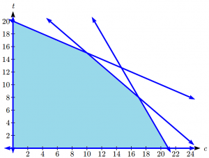

There are five corner points for this region.

Point 1: In the lower left, where t = 0 crosses c = 0. Point: (0, 0)

Point 2: In the upper left, where c = 0 crosses $c+2t=40$ .
Using substitution, $2t=40$ , so t = 20.
Point: (0, 20)

Point 3: In the lower right, where t = 0 crosses $2c+t=42$ .
Using substitution, $2c=42$ , so c = 21.
Point: (21, 0)

Point 4: The solution to the system:
$c+2t=40$
$c+t=25$
So multiply the second equation by -1 and add:
$\begin{array}{r} c+2t=40\\ -c-t=-25\\ \hline t=15 \end{array}$
Substitute to find $c$ : $c+15=25$ so $c=10$
Point: (10,15)

Point 5: The solution to the system:
$2c+t=42$
$c+t=25$
So multiply the bottom equation by -1 and add:
$2c+t=42\\ -c-t=-25\\ \hline c=17 \end{array}$
Substitute to find $t$ : $17+t=25$ so $t=8$
Point: (17,8)

Testing the objective function at each of these corner points:

Point	Profit, P = 20c + 30t
(0, 0)	P = 20(0) + 30(0) = $0
(0, 20)	P = 20(0) + 30(20) = $600
(21, 0)	P = 20(21) + 30(0) = $420
(10, 15)	P = 20(10) + 30(15) = $650
(17, 8)	P = 20(17) + 30(8) = $580

The profit will be maximized by producing 10 chairs and 15 tables.

Graphing is not the only way to do Linear Programming and Optimization. There is another method, called The Simplex Method. It is included in the source material for this chapter. Most people use technology for these problems as well and many can be found online. While this books gives only an introduction to Linear Programming, it is used in many business applications.

Try it Now Answers

Max $P=14x+9y$

subject to:
$x+y \leq 9$
$3x +y \leq 15$
$x \geq 0, y \geq 0$

Graphing the feasible region, we see there are three corner points of potential interest: (0, 9), (5, 0), and the intersection of the two lines at (3, 6). We then evaluate the objective function at each corner point.

Try it Now 1 Graph

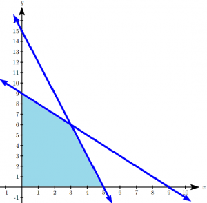
Point
(0, 9)	81
(5, 0)	70
(3, 6)	96

$P$ is maximized when $x=3, y=6$ .

2. Let a be the number of product A produced, and b be the number of product B.

Our goal is to maximize profit: $P=50a+60b$

From manufacturing we get the constraints:
$3a+4b \leq 84$

From assembly we get the constraint:
$1a+2b \leq 32$

We have corner points at (0,16), (28,0). The third is at the intersection of the two lines. To find that we could multiply the second equation by -2 and add:
$\begin{array}{r} 3a + 4b = 84\\ - 2a - 4b = - 64\\ \hline a=20 \end{array}$
The third corner point (20,6).

Evaluating the objective function at each of these points:

Point

P

(0, 16)

P = 50(0) + 60(16) = 960

(28, 0)

P = 50(28) + 60(0) = 1400

(20, 6)

P = 50(20) + 60(6) = 1360

Profit will be maximized by producing 28 units of product A and 0 units of product B.

Media Attributions

linearprogexample1
linearprogexample2
linearprogexample3
takenote is licensed under a Public Domain license
linearprogexample4
linearprogexample5
tin421

License

Icon for the Creative Commons Attribution-ShareAlike 4.0 International License

Media Attributions

License

Share This Book