4.1 Linear Inequalities in Two Variables

Terri Manthey

4.1 Linear Inequalities in Two Variables

A linear equation in two variables is an equation like $f(x)=2x+1$ , which is sometimes written without function notation as $y=2x+1$ . Recall that the graph of this equation is a line, formed by all the points $(x,y)$ that satisfy the equation.

A linear inequality in two variables is similar, but involves an inequality. Some examples:

$y<2x+1 \quad y>4x-1 \quad y\leq \dfrac{2}{3}x+4 \quad y\geq 5-2x$

Linear inequalities can also be written with both variables on the same side of the equation, like $2x-3y<4$

The solution set to a linear inequality will be all the points $(x,y)$ that satisfy the inequality. Notice that the line $y=2x+1$ divides the coordinate plane into two halves; on one half $y<2x+1$ , and on the other $y>2x+1$ . The solution set to a linear inequality will be a half-plane, and to show the solution set we shade part of the coordinate plane where the points lie in the solution set.

To Graph the Solution to a Linear Inequality

If necessary, rewrite the linear inequality into a form convenient for graphing, like slope-intercept form.
Graph the corresponding linear equation.
1. For a strict inequality (< or >), draw a dashed line to show that the points on the line are not part of the solution
2. For an inequality that includes the equal sign ( $\leq$ or $\geq$ ), draw a solid line to show that the points on the line are part of the solution.
Choose a test point, not on the line. (0,0) or (0,1) are the easiest!
1. Substitute the test point into the inequality
2. If the inequality is true at the test point, shade the half plane on the side including the test point
3. If the inequality is not true at the test point, shade the half plane on the side that doesn’t include the test point.

Example of Graphing the Solutions of a Linear Inequalities

a. Graph the solution to 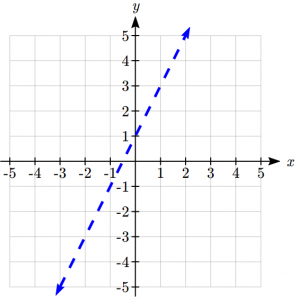$y<2x+1$ Graph of y=2x+1 with dotted line

Since this is a strict inequality, we will graph $y=2x+1$ as a dashed line.

Now we choose a test point not on the line, like (0,0).

Substituting (0,0) into the inequality, we get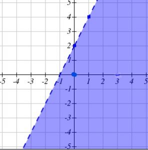 Graph of y<2x+1
$0<2(0)+1$
$0<1$

This is a true statement, so we will shade the side of the plane that includes (0,0).

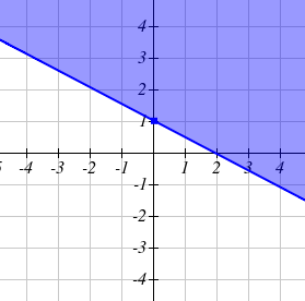
b. Graph the solution to $x \geq 2y+4$

This is not written in a form we are used to using for graphing, so we might solve it for $y$ first. graph of y=-2+1/2x

$\begin{array}{l} x \geq 2y+4\\ x-2y \geq 4\\ -2y \geq 4-x\\ y \leq -2+ \dfrac{1}{2}x \end{array}$

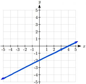
Since this inequality includes the equals sign, we will graph $y=-2+\dfrac{1}{2}x$ as a solid line. Graph of y

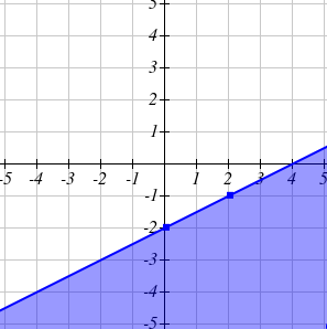
Now we choose a test point not on the line. (0,0) is a convenient choice. Substituting (0,0) in the inequality, we get

$\begin{array}{l} 0 \geq 2(0) +4\\ 0 \geq 4\end{array}$ NO!

Since this is a false statement, we shade the half of the plane that does not include (0,0).

Try it Now 1

Graph the solution to $y \geq -\dfrac{1}{2}x+1$

Example of Applications of Linear Equalities

A store sells peanuts for $4/pound and cashews for $8/pound, and plans to sell a new mixed-nut blend in a jar. What combinations of peanuts and cashews are possible, if they want the mix to cost $6 or less?

We start by defining our variables:
$p$ : The number of pounds of peanuts in 1 pound of mix
$c$ : The number of pounds of peanuts in 1 pound of mix

The cost of one pound of mix will be $4p+8c$ , so all the mixes costing $6 or less will satisfy the inequality $4p+8c \leq 6$ .

We can graph the equation $4p+8c=6$ fairly easily by finding the intercepts:
When $p=0$ ,
$8c=6$
$c=\dfrac{3}{4}$
Which means we have a point $\left(0, \dfrac{3}{4} \right)$ is on the line. Graph of 4p+8c<=6 and x,y >=0

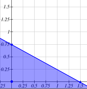
When $c=0$
$4p=6$
$p=\dfrac{3}{2}$
So we have the point $\left(\dfrac{3}{4},0 \right)$

Notice the test point (0,0) will satisfy the inequality, $0+0 \leq 6$ so we will shade the side of the line including the origin. Because of the context , only values in the first quadrant are reasonable. The graph shows all the possible combinations the store could use, including 1 pound of peanuts with 1/4 pound of cashews, or 1/2 a pound of each.

Systems of Linear Inequalities

In the systems of equations chapter, we looked for solutions to a system of linear equations – a point that would satisfy all the equations in the system. Likewise, we can consider a system of linear inequalities. The solution to a system of linear inequalities is the set of points that satisfy all the inequalities in the system.

With a single linear inequality, we can show the solution set graphically. Likewise, with a system of linear inequalities we show the solution set graphically. We find it by looking for where the regions indicated by the individual linear inequalities overlap.

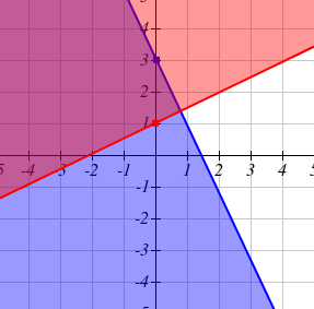
Example of a System of Linear Inequalities

Graph the solution to the system of linear inequalities
$\begin{array}{l} y \leq x+2\\ y \geq 1-x\end{array}$

We can look at graphs of each of the inequalities, but the best way is to graph the solution sets on the same axes reveals the solution to the system of inequalities as the region where the two overlap. You can erase the parts that are only covered once to show the solution set.

With technology, there are some calculators that will graph linear inequalities. Desmos can do this if you type in the $y <$ or $y \geq$ . For systems you can actually put them on the same line with the second one in brackets and it will graph just the solution set of the system. For the example above this is $y \leq x+2$ { $y \geq 1-x$ }.

Try it Now 2

Graph the solution to the system of linear inequalities

$\begin{array}{l} y \leq 3-2x\\ y \geq \dfrac{1}{2}x+1\end{array}$

The following question is similar to a problem we solved using systems in the systems chapter.

Example of an Application of Systems of Inequalities

A company produces a basic and premium version of its product. The basic version requires 20 minutes of assembly and 15 minutes of painting. The premium version requires 30 minutes of assembly and 30 minutes of painting. If the company has staffing for 3,900 minutes of assembly and 3,300 minutes of painting each week. How many items can then produce within the limits of their staffing?

Notice this problem is different than the question we asked in the first section, since we are no longer concerned about fully utilizing staffing, we are only interested in what is possible. As before, we’ll define b: The number of basic products made, p: The number of premium products made.

Just as we created equations in the first section, we can now create inequalities, since we know the hours used in production needs to be less than or equal to the hours available. This leads to two inequalities:

$\begin{array}{l} 20b+30p \leq 3900\\ 15b+30p \leq 3300 \end{array}$

Graphing these inequalities gives us the solution set. 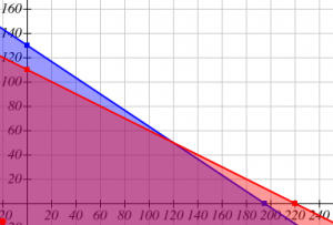Graph of the system 20b+30p <=3900 and 15b+30p<=3300 in first quadrant

Since it isn’t reasonable to consider negative numbers of items, we can further restrict the solutions to the first quadrant. This could also be represented by adding the inequalities $b \geq 0, p \geq 0$ .

In the solution set we can see the solution to the system of equations we solved in the previous section: 120 basic products and 50 premium products. The solution set shows that if the company is willing to not fully utilize the staffing, there are many other possible combinations of products they could produce.

The techniques we used above are key to a branch of mathematics called linear programming, which is used extensively in business. We will explore linear programming further in the next section.

Try it Now Answers

Media Attributions

inequalityegstep1
inequalityegstep2_LI
inequalityeq2step1_LI
inequalityeq2step2
ineqexampapp
ineqsystemeg
tinanswer411
tinanswer412

License

Icon for the Creative Commons Attribution-ShareAlike 4.0 International License

Systems of Linear Inequalities

Media Attributions

License

Share This Book