
5.3 Higher Order Polynomials
In the previous section we explored the short run behavior of quadratics, a special case of polynomials. In this section we will explore the behavior of polynomials in general. The basic building blocks of polynomials are power functions.
Power Function
A power function is a function that can be represented in the form

Where the base is a variable and the exponent, p, is a number.
Characteristics of Power Functions
Shown to the right are the graphs of  , and
, and  , all even
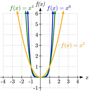 whole number powers. Notice that all these graphs have a fairly similar shape, very similar to a quadratic, but as the power increases the graphs flatten somewhat near the origin, and become steeper away from the origin.
To describe the behavior as numbers become larger and larger, we use the idea of infinity. The symbol for positive infinity is  , and
, and  for negative infinity. When we say that “x approaches infinity”, which can be symbolically written as
  , we are describing a behavior – we are saying that
  is getting large in the positive direction.
With the even power function, as the input becomes large in either the positive or negative direction, the output values become very large positive numbers. Equivalently, we could describe this by saying that as approaches positive or negative infinity, the  values approach positive infinity. In symbolic form, we could write: as
  ,
,  .
.
Shown here are the graphs of  , and
, and  , all odd whole
 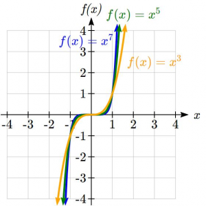 number powers. Notice all these graphs look similar, but again as the power increases the graphs flatten near the origin and become steeper away from the origin.
For these odd power functions, as approaches negative infinity, approaches negative infinity. As approaches positive infinity, approaches positive infinity. In symbolic form we write: as  ,
,  and as , .
Long Run Behavior
The behavior of the graph of a function as the input takes on large negative values () and large positive values () as is referred to as the long run behavior of the function.
Polynomials
Recall our definitions of polynomials from chapter 1.
Terminology of Polynomial Functions
A polynomial is function that can be written as 
Each of the  constants are called coefficients and can be positive, negative, or zero, and be whole numbers, decimals, or fractions.
A term of the polynomial is any one piece of the sum, that is any  . Each individual term is a transformed power function.
The degree of the polynomial is the highest power of the variable that occurs in the polynomial.
The leading term is the term containing the highest power of the variable: the term with the highest degree.
The leading coefficient is the coefficient of the leading term.
Because of the definition of the “leading” term we often rearrange polynomials so that the powers are descending.

For any polynomial the long run behavior of the polynomial will match the long run behavior of the leading term.
Example of Polynomial Graph
What can we determine about the long run behavior and degree of the equation for the polynomial graphed here?
Since the output grows large and positive as the inputs grow large and positive, we describe the long run behavior symbolically by writing: as , . Similarly, as , .
In words, we could say that as x values approach infinity, the function values approach infinity, and as x values approach negative infinity the function values approach negative infinity.
We can tell this graph has the shape of an odd degree power function which has not been reflected, so the degree of the polynomial creating this graph must be odd, and the leading coefficient would be positive.
Short Run Behavior: Intercepts
Characteristics of the graph such as vertical and horizontal intercepts and the places the graph changes direction are part of the short run behavior of the polynomial.
Like with all functions, the vertical intercept is where the graph crosses the vertical axis, and occurs when the input value is zero. Since a polynomial is a function, there can only be one vertical intercept, which occurs at the point  . The horizontal intercepts occur at the input values that correspond with an output value of zero. It is possible to have more than one horizontal intercept.
Horizontal intercepts are also called zeros, or roots of the function.
To find horizontal intercepts, we need to solve for when the output will be zero. For general polynomials, this can be a challenging prospect. While quadratics can be solved using the relatively simple quadratic formula, the corresponding formulas for cubic and 4th degree (also called quartic) polynomials are not simple enough to remember, and formulas do not exist for general higher-degree polynomials. In the next section, we will explore a few more techniques for finding roots of cubic and quartic functions, but for this section we will restrict the discussion to cubic and quartic functions in which:
- The polynomial can be factored using known methods: greatest common factor, trinomial factoring or factoring by grouping.
- The polynomial is given in factored form.
- Technology is used to determine the intercepts. (i.e. your calculator or Desmos)
Examples Finding Horizontal Intercepts by Factoring
a. Find the horizontal intercepts of 
Let’s try factoring this polynomial to find solutions for  .
.
Remember the first thing we always want to do when factoring is to see if we can factor out a GCF:
We see that every term contains 

 Now what we have left is a quadratic form. This means that we see that we have a trinomial in which the variable part of one term is the square of another and those are the only two variable parts.
Notice that  So we can factor the trinomial as quadratic form.

Now we can break these apart to solve:

We have 5 horizontal intercepts: 
b. Find the vertical and horizontal intercepts of 
The vertical intercept can be found by evaluating  .
.

The horizontal intercepts can be found by solving 

Since this is already factored we can break it apart:

c.Find the horizontal intercepts of 
Since this polynomial is not in factored form, has no common factors, and does not appear to be factorable using techniques we know, we can turn to technology to find the intercepts.
Going to Desmos for this graph, we can see: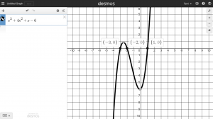
By clicking on the grey dots on the axis, we see the horizontal intercepts are (-3,0), (-2,0) and (1,0).
We could check these are correct by plugging in these values for t and verifying that  .
.
Notice that the polynomial in the previous example, part c was degree three, and had three horizontal intercepts and two turning points – places where the graph changes direction. However, part b was also cubic and had 2 intercepts, while the degree 6 polynomial in a had 5. We will now make a general statement without justifying it.
Intercepts and Turning Points of Polynomials
A polynomial of degree  will have:
- At most horizontal intercepts. An odd degree polynomial will always have at least one.
- At most
 turning points.
Try it Now 1
Find the vertical and horizontal intercepts of the function 
Graphical Behavior at Intercepts
If we graph the function 
 , notice that the behavior at each of the horizontal intercepts is different.
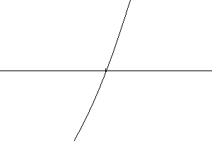
At the horizontal intercept  , coming from the
  of the polynomial, the graph passes directly through the horizontal intercept. The factor is linear (has a power of 1), so the behavior near the intercept is like that of a line – it passes directly through the intercept. We call this a single zero, since the zero corresponds to a single factor of the function.
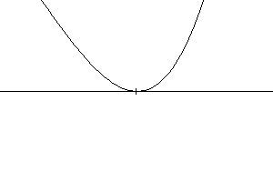
At the horizontal intercept  , coming from the
  factor of the polynomial, the graph touches the axis at the intercept and changes direction. The factor is quadratic (degree 2), so the behavior near the intercept is like that of a quadratic – it bounces off of the horizontal axis at the intercept. Since
  , the factor is repeated twice, so we call this a double zero. We could also say the zero has multiplicity 2.
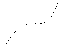
At the horizontal intercept  , coming from the factor
  of the polynomial, the graph passes through the axis at the intercept, but flattens out a bit first. This factor is cubic (degree 3), so the behavior near the intercept is like that of a cubic, with the same “S” type shape near the intercept as
  . We call this a triple zero. We could also say the zero has multiplicity 3.
By utilizing these behaviors, we can sketch a reasonable graph of a factored polynomial function without needing technology. We might want to do that because it is very easy to make a typing mistake in Desmos and especially a graphing calculator. It is very important to have an understanding of what a graph should look like in order to know that you have typed in the function you are graphing correctly.
Graphical Behavior of Polynomials at Horizontal Intercepts
If a polynomial contains a factor of the form  , the behavior near the horizontal intercept h is determined by the power on the factor.
For higher even powers 4,6,8 etc.… the graph will still bounce off of the horizontal axis but the graph will appear flatter with each increasing even power as it approaches and leaves the axis.
For higher odd powers, 5,7,9 etc… the graph will still pass through the horizontal axis but the graph will appear flatter with each increasing odd power as it approaches and leaves the axis.
Example Sketching a Graph
Sketch a graph of  .
.
This graph has two horizontal intercepts. At , the factor is squared, indicating the graph will bounce at this horizontal intercept. At  , the factor is not squared, indicating the graph will pass through the axis at this intercept.
Additionally, we can see the leading term, if this polynomial were multiplied out, would be -2x^3, so the long-run behavior is that of a vertically reflected cubic, with the outputs decreasing as the inputs get large positive, and the inputs increasing as the inputs get large negative. In other words, this ends down on on the right side and up on the right side.
To sketch this we consider the following:
As , the function so we know the graph starts in the 2nd quadrant and is decreasing toward the horizontal axis.
At (-3, 0) the graph bounces off of the horizontal axis and so the function must start increasing.
At (0, 90) the graph crosses the vertical axis at the vertical intercept. This is obtained by plugging 0 in 
Somewhere after this point, the graph must turn back down or start decreasing toward the horizontal axis since the graph passes through the next intercept at (5,0).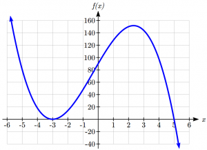
As the function so we know the graph continues to decrease and we can stop drawing the graph in the 4th quadrant.
Using technology we can verify that the resulting graph will look like:
Try it Now 2
Given the function  use the methods that we have learned so far to find the vertical & horizontal intercepts, determine where the function is negative and positive, describe the long run behavior and sketch the graph without technology.
We can also use what we know to make guesses about a graph of a polynomial. [1]
Example using a Graph to Learn about a Polynomial
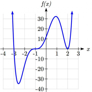
What can you learn about this polynomial from the graph? 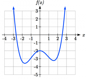
Based on the long run behavior, with the graph becoming large positive on both ends of the graph, we can determine that this is the graph of an even degree polynomial. The graph has 2 horizontal intercepts, suggesting a degree of 2 or greater, and 3 turning points, suggesting a degree of 4 or greater. Based on this, it would be reasonable to conclude that the degree is even and at least 4, so it is probably a fourth degree polynomial.
The previous example was difficult to tell the exact zeros since they were not integers, but often, we can actually find the equation for a graphed polynomial.
Example using a Graph to write the equation for a Polynomial
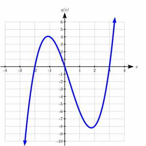
Write a formula for the polynomial function graphed here.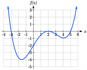
This graph has three horizontal intercepts: x = -3, 2, and 5. At x = -3 and 5 the graph passes through the axis, suggesting the corresponding factors of the polynomial will be linear to power 1. At x = 2 the graph bounces at the intercept, suggesting the corresponding factor of the polynomial will be squared. We also notice that the graph rises on both sides and has 3 turn-around points, so it appears to be degree 4. Also, we do not know the coefficient in the front of the lead term, a, at this point. So far, we know:

To determine the lead coefficient (also known as a stretch factor), we can utilize another point on the graph. Here, we see the vertical intercept appears to be  so we can plug those values to solve for a.

The graphed polynomial appears to represent the function

Try it Now 3
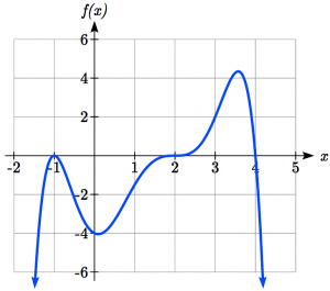
Given the graph, write a formula for the function shown.
Finding Extrema
With quadratics, we were able to algebraically find the maximum or minimum value of the function by finding the vertex. For general polynomials, finding these turning points is not possible without more advanced techniques from calculus. Even then, finding where extrema occur can still be algebraically challenging. For now, we will estimate the locations of turning points using technology to generate a graph.
- In Desmos, maximum and minimum values have a grey dot that can be clicked on to determine the maximum and minimum values
- Instructions on a TI 83/84 and Casio for find relative maximums and minimums
Example Maximizing a Higher Order Polynomial Function
An open-top box is to be constructed by cutting out squares from 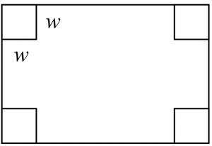 each corner of a 14cm by 20cm sheet of plastic then folding up the sides. Find the size of squares that should be cut out to maximize the volume enclosed by the box.
We will start this problem by drawing a picture, labeling the width of the cut-out squares with a variable, w.
Notice that after a square is cut out from each end, it leaves a  cm by
cm by  cm rectangle for the base of the box, and the box will be
  cm tall. This gives the volume:

Using technology to sketch a graph allows us to estimate the maximum value for the volume, restricted to reasonable values for w: values from 0 to 7.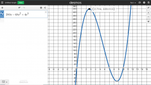
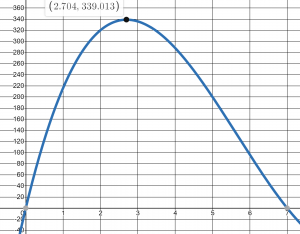
From this graph, we can find the maximum value at 339.013, and occurs when the squares are about 2.704cm square.
Try it Now 4
Use technology to find the maximum and minimum values on the interval [-1, 4] of the function  .
.
Try it Now Answers
- Vertical intercept
 , Horizontal intercepts
- Vertical intercepts , Horizontal intercepts

The function is negative on and
and 
The function is positive on and
and 
The leading term is so as
so as  and as
- Double zero at
 , triple zero at
  , single zero at
  .
.

Substitute (0,4) and solve for :
: 
- The minimum occurs at approximately the point (0, -6.5), and the maximum occurs at approximately the point (3.5, 7).
Media Attributions
- evenpowers
- oddpowers
- takenote is licensed under a Public Domain license
- 53example2
- behaviorofgraphatintercepts
- triplezero
- singlezero
- doublezero
- 53example3
- 53example5
- 53example6
- tin533
- examplebox
- 53example4
- zoomedingraph534
- tin532
- The next two examples and Try it Now is from Precalculus: An Investigation of Functions by Lippman and Rasmussen, Licensed under Creative Commons 4.0, CC-BY-SA ↵
